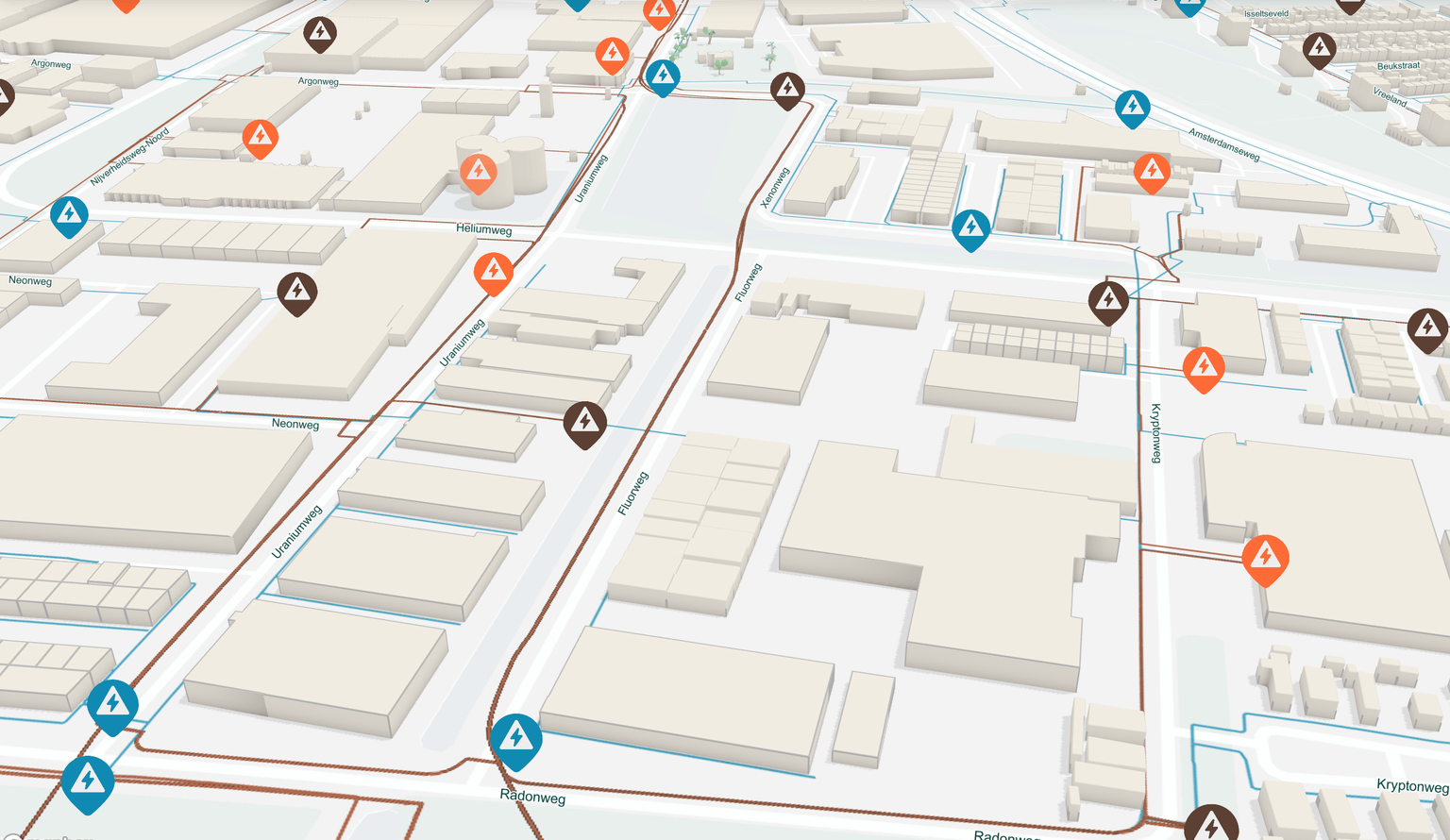
Focal Grid

TL;DR

Built a full-stack GIS platform for visualizing Dutch energy grid data using Nuxt, Mapbox, Supabase, and PostGIS. Implemented a GeoJSON ingestion pipeline, custom map interactions, and a performant vector tile backend that serves geospatial data directly from PostGIS while keeping Mapbox purely as the rendering engine.

Mini Demo

Background

While working full-time on freelance full-stack projects got in contact with a client looking to build a GIS-based visualisation platform. The pitch was straightfoward, in service of energy grid buildout in the Netherlands many private providers are looking to efficiently aggregate data in order make decisions on planning, contracts, budgets, etc. The goal was to build a minimum viable web-based prototype that demonstrates the basic desired visualisation and interaction funcionallity to show to stakeholders. Taking on the challenge as a solo developer, this was one of my most impactful freelance projects seeing as it steered me to GIS engineering for the very first time.

Tech Stack

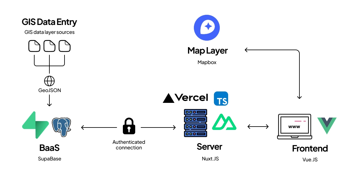
The application follows a fairly straightforward full-stack architecture. The frontend is built with Nuxt and Vue, which pair nicely with the Mapbox GL JS SDK while also giving me a framework I'm comfortable moving quickly in. Since almost all application data is user-specific and fetched on demand, there was little reason to lean on SSR beyond the initial page shell.

On the backend I used Supabase as the primary BaaS solution. Besides hosting a PostGIS-enabled PostgreSQL database, it also provided authentication and Edge Functions for serving vector tiles directly from the database. This let Mapbox handle rendering while keeping the actual geospatial data entirely outside of the Mapbox ecosystem.

The project itself was deployed on Vercel, with TypeScript used throughout both the frontend and server code. Finally, GSAP was sprinkled in for a handful of subtle interface animations, mostly around menus and transitions without becoming a central part of the application.

Key Features

Custom UI & Map Interactions

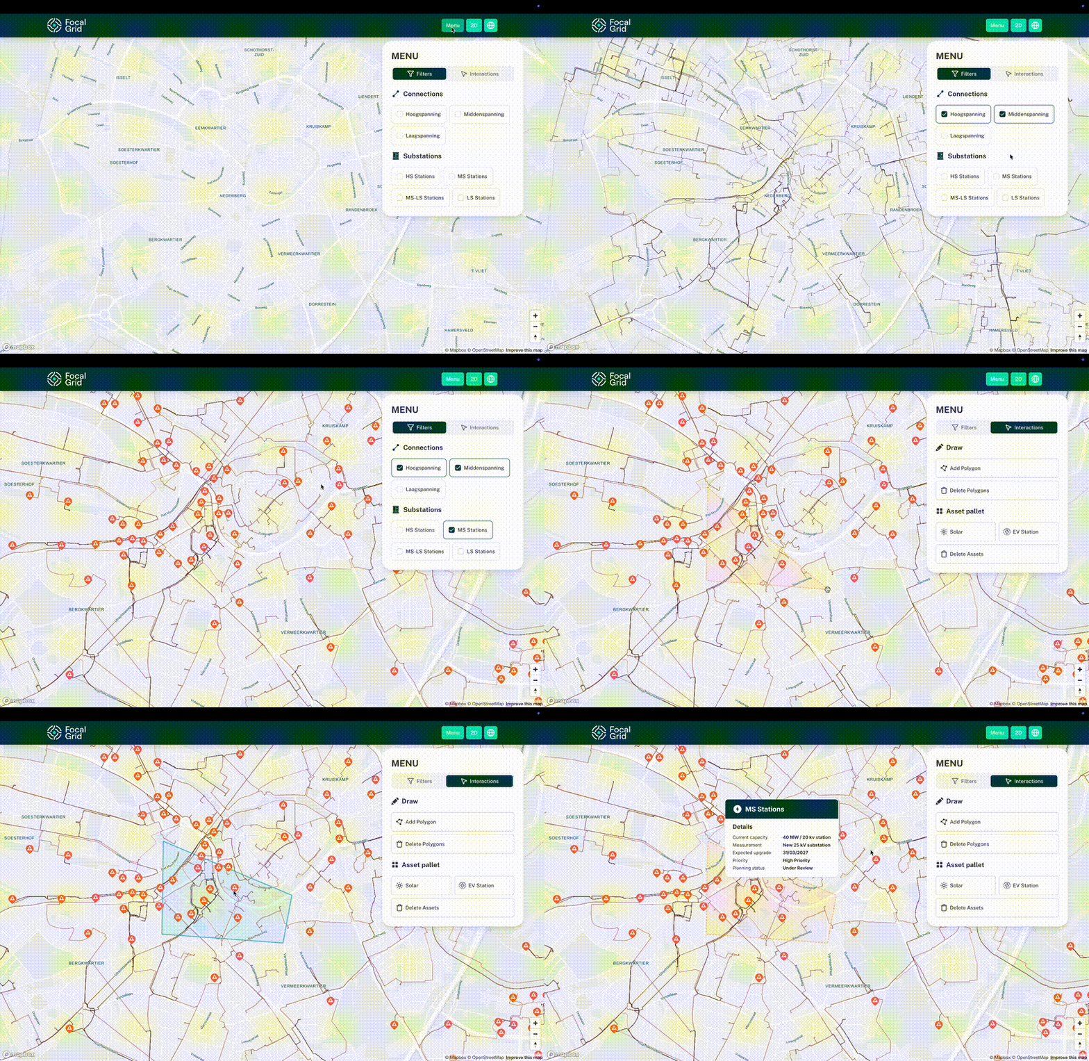
Perhaps this might be the easiest part to grasp intuitively seeing the Mini Demo above already reveals most of the built functionality. Still, it might be good to list out the available features after concluding my work. The app largely consists of, number one, a interactive map render component, and two, a header component offering different control options. Controls offered by the popover menu include:

• Toggling different energy grid layers on and off which were seperated by their voltage;
• Toggling energy substations connected to each kind of voltage level;
• On-map polygon drawing and deletion for grouping data points geographically;
• Drag-and-drop icons for projecting energy asset placement;

Furthermore, the top bar additionally includes simple sattelite view and pitched angle toggle buttons.

When talking about the map itself, the user is able to zoom and inspect a limited geographical area (in this case Amersfoort in the Netherlands) as you might expect from any other map-based web application. On top of that, user can click on substations to dynamically load and view the stations metadata.

From a technical standpoint, most of the interaction logic lives in small Vue composables that bridge UI state to Mapbox through some SDK-provided hooks. The trickiest part for me was definetily keeping all of this stable across style reloads. Switching between the custom basemap and satellite view tears down and rebuilds Mapbox layers. This forced me to add special hooks to re-sync restore connection layers and persist drawn points in memory before re-injecting them after the style loads.

GeoJSON to PostGIS Pipeline

The data source for the energy grid related data was open data provided by the municipality of Amersfoort. At the time, only data in GeoJSON format was available. This meant that I needed to find a reliable way in which import this data directly into a Postgres table in Supabase while maintaining the usability of the data.

I landed on the following helper function. Provided with a local file path, desired table name and Supabase client object it automatically loads the GeoJSON into a PostGIS compatible Supabase table.

async function importGeoJSON(
  filePath, 
  tableName, 
  supabaseClient
) {
  try {
    const geojson = JSON.parse(fs.readFileSync(filePath, 'utf8'))
    
    // Process in batches to avoid timeouts
    const batchSize = 1000
    const features = geojson.features.map(feature => ({
      geom: feature.geometry,
      properties: feature.properties || {}
    }))

    console.log(`Importing ${features.length} features...`)
    
    for (let i = 0; i < features.length; i += batchSize) {
      const batch = features.slice(i, i + batchSize)
      const { data, error } = await supabaseClient
        .from(tableName)
        .insert(batch)
      
      if (error) {
        console.error('Error inserting batch:', error)
        break
      }
      
      console.log(`Inserted batch ${Math.floor(i/batchSize) + 1}/${Math.ceil(features.length/batchSize)}`)
    }
    
    console.log('Import completed!')
  } catch (error) {
    console.error('Import failed:', error)
  }
}

This function can work perfectly as an Edge Function. However, for the sake of the "minimum viable" aspect of the project I just ran it as a local Node.JS application

Dynamic Vector Tile Querying

Early on the client mentioned the desire to use Mapbox styling on the frontend while avoiding vendor lock-in risks on the data storage. This posed an interesting challenge to me, namely, 'how can I render map layers natively on the frontend while keeping the data completely external to Mapbox?'. Lucky for me, Mapbox allows for querying external sources by sending simple HTTP requests to a given endpoint using the users current bounding box in the query parameters (example later on). The response has to conform to the Mapbox Vector Tile specification (basically Google's Protocol Buffer format).

Using Supabase made things slighlty easier. Using their Edge Functions I could quickly setup a read-only endpoint to receive the incoming Mapbox requests. This Edge Function internally calls an RPC function which does the heavy lifting in terms of geometry fetching and processing. Below you can see a simplified outline main Edge Function body. Notice how I added a custom query parameter allowing for a dynamic dataset selection.

serve(async (req)=>{
  // Parses query parameters from url 
  // example: /functions/mvt/dataset123/{z}/{x}/{y}
  const url = new URL(req.url);
  const parts = url.pathname.split('/').filter((p)=>p.length > 0);
  const mvtIndex = parts.indexOf('mvt');
  const dataset = parts[mvtIndex + 1];
  const z = Number(parts[mvtIndex + 2]);
  const x = Number(parts[mvtIndex + 3]);
  const y = Number(parts[mvtIndex + 4]);

  // Calls supabase RPC function to query the actual geo data
  // Args are parsed earlier from query parameters
  const { data: vectorTileBinary, error } = await supabase.rpc('get_dynamic_lines_mvt', {
    dataset,
    z,
    x,
    y
  });
 
  // Returns mvt data in raw bytes
  return new Response(vectorTileBinary, {
    status: 200,
    headers: {
      ...corsHeaders,
      'Content-Type': 'application/vnd.mapbox-vector-tile'
    }
  });
});

Now for the interesting part. The PostgreSQL get_dynamic_lines_mvt RPC function was made to have very rudamentary API, as shown below:

CREATE OR REPLACE FUNCTION public.get_dynamic_lines_mvt(
  dataset text,
  z integer,
  x integer,
  y integer
) RETURNS bytea

What actually happens inside of the function body can best be described in a handful of procedural steps.

Firstly, the sent coordinates values (x, y, z) are translated into rectangular polygon coordinates representing the user's bounding box.

bounds3857 := ST_TileEnvelope(z, x, y);

Next, geometries that land outside of the requested tile are filtered out before moving on to expensive intersection computations.

WITH filtered AS (
  SELECT ST_Transform(wkb_geometry, 3857) AS geom3857 FROM %I.%I
  WHERE ST_Transform(wkb_geometry, 3857) && $1::geometry
  AND ST_Intersects(ST_Transform(wkb_geometry, 3857), $1::geometry)
),

To further help performance, before any of the expensive geometry checks are done, the caller's z-value gets evaluated and classified. This is done in oreder to not overfetch very detailed geometry data for a large zoomed-out bounding box when geometry resolution is least important.

simplification := CASE
  WHEN z <= 5  THEN 80
  WHEN z <= 10 THEN 15
  ELSE 0
END;

This value is subsequently used as an argument to clip and simplify the data to varying degrees. At the same time, ST_AsMVTGeom turns the simplified geometries from "Well-Known Binary" representation found in the actual table into the coordinate space of a MVT tile stored in mvtgeom.

mvtgeom AS (
  SELECT
    ST_AsMVTGeom(
      CASE
        WHEN $2 > 0
          THEN ST_SimplifyPreserveTopology(geom3857, $2)
        ELSE geom3857
      END,
      $1, 4096, 0, true
    ) AS geom
  FROM filtered
)

Finally, filtered and simplified data is serialized into raw mvt bytes to be returned to the caller and later the user.

SELECT ST_AsMVT(
  q,
  'lines',
  4096,
  'geom'
)
FROM (
  SELECT geom
  FROM mvtgeom
) q;

As you may already have noticed, in order to achieve much of the geometry translation and serialization functionallity I made use of PostGIS' exhaustive list of Special Functions. Perhaps this post is not the ideal place to go into detail on them so I highly recommend checking out the official PostGIS Special Function Index in case you'd like to know more. The main Special Functions I ended up using were the following:

ST_TileEnvelope()
ST_Transform()
ST_SimplifyPreserveTopology()
ST_Intersects()
ST_AsMVTGeom()
ST_AsMVT()